Every developer who touches a backend, runs a data migration, or debugs a production issue will eventually need to write or read SQL. It is not optional knowledge - databases power almost every application, and SQL is how you talk to them.
This guide covers the core SQL queries you need to know as a developer: how to fetch data, filter it, sort it, aggregate it, join tables, and modify records. Each section uses a consistent example schema so the queries build on each other naturally. If you want to understand why relational databases are structured this way before diving into queries, start with Relational Databases Explained: Tables, Rows, and Keys.
Table of Contents
Open Table of Contents
- The Example Schema
- SELECT: Fetching Data
- WHERE: Filtering Rows
- ORDER BY and LIMIT: Sorting and Paging
- INSERT: Adding Records
- UPDATE: Modifying Records
- DELETE: Removing Records
- Aggregate Functions: COUNT, SUM, AVG, MIN, MAX
- GROUP BY: Summarizing Data
- JOIN: Combining Tables
- Common Mistakes Beginners Make
- Interview Questions
- 1. What is the difference between WHERE and HAVING?
- 2. What is the difference between INNER JOIN and LEFT JOIN?
- 3. Why is SELECT * considered bad practice?
- 4. What happens if you run DELETE without a WHERE clause?
- 5. What is the difference between COUNT(*) and COUNT(column)?
- 6. What is the query execution order in SQL?
- Conclusion
- References
- YouTube Videos
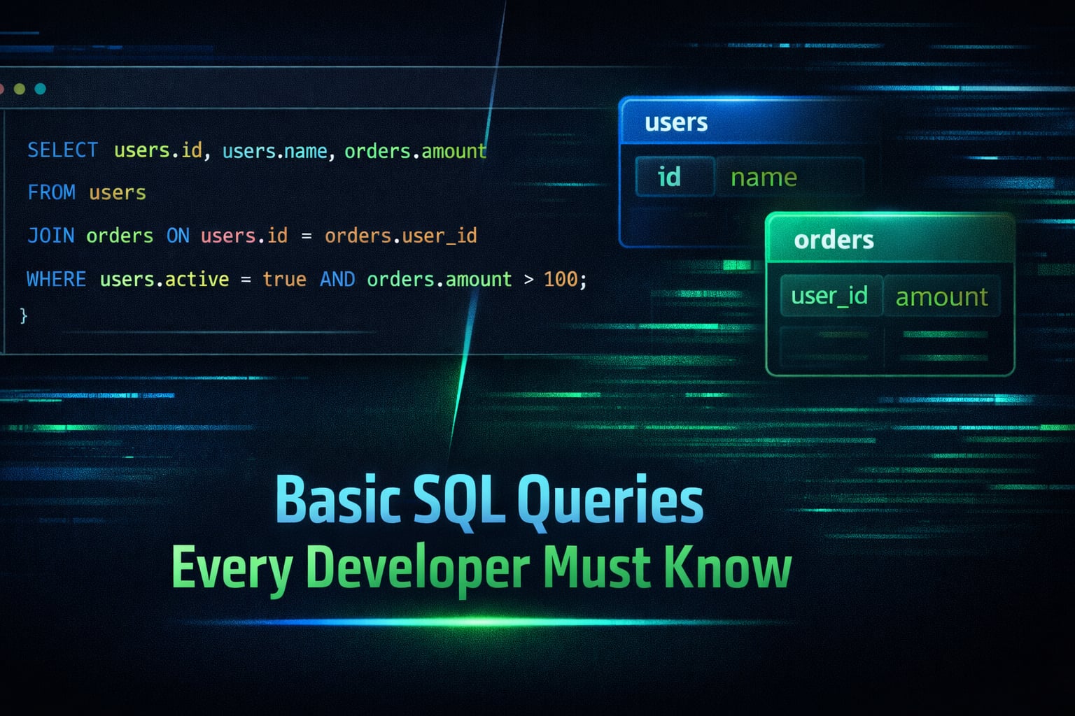
The Example Schema
All queries in this guide use two tables: users and orders. This keeps examples grounded and shows how queries connect across tables.
-- users table
CREATE TABLE users (
  id       INT PRIMARY KEY,
  name     VARCHAR(100),
  email    VARCHAR(150),
  country  VARCHAR(50),
  joined   DATE
);

-- orders table
CREATE TABLE orders (
  id         INT PRIMARY KEY,
  user_id    INT,
  product    VARCHAR(100),
  amount     DECIMAL(10, 2),
  status     VARCHAR(20),
  created_at DATE
);
Sample data to picture as you read:
| id | name | country | joined | |
|---|---|---|---|---|
| 1 | Alice Chen | alice@example.com | USA | 2023-01-15 |
| 2 | Bob Martins | bob@example.com | UK | 2023-03-22 |
| 3 | Carol Davis | carol@example.com | USA | 2024-06-10 |
| 4 | David Lee | david@example.com | Canada | 2024-09-01 |
| id | user_id | product | amount | status | created_at |
|---|---|---|---|---|---|
| 1 | 1 | Laptop | 999.00 | completed | 2024-01-10 |
| 2 | 1 | Mouse | 25.00 | completed | 2024-02-14 |
| 3 | 2 | Keyboard | 75.00 | pending | 2024-03-05 |
| 4 | 3 | Monitor | 350.00 | completed | 2024-04-20 |
| 5 | 4 | Headphones | 120.00 | cancelled | 2024-05-01 |
SELECT: Fetching Data
SELECT is the most fundamental SQL statement. Every data-reading query starts with it.
Fetch all columns
SELECT * FROM users;* means “all columns.” This works fine for exploration but avoid it in production code - fetching unnecessary columns wastes bandwidth and makes queries harder to read.
Fetch specific columns
SELECT name, email FROM users;Result:
| name | |
|---|---|
| Alice Chen | alice@example.com |
| Bob Martins | bob@example.com |
| Carol Davis | carol@example.com |
| David Lee | david@example.com |
Column aliases with AS
AS renames a column in the output without changing the table.
SELECT name AS full_name, email AS contact FROM users;DISTINCT: Unique values only
SELECT DISTINCT country FROM users;Result: USA, UK, Canada - duplicates removed.
WHERE: Filtering Rows
WHERE filters which rows are returned. It goes after FROM and before ORDER BY.
Basic comparison
SELECT * FROM users WHERE country = 'USA';Returns Alice and Carol only.
Common WHERE operators
-- Equal / not equal
WHERE status = 'completed'
WHERE status != 'cancelled'

-- Numeric comparisons
WHERE amount > 100
WHERE amount BETWEEN 50 AND 200

-- Text pattern matching (% = any characters, _ = one character)
WHERE name LIKE 'A%'       -- starts with A
WHERE email LIKE '%@example.com'

-- Match a list of values
WHERE country IN ('USA', 'Canada')

-- NULL checks
WHERE joined IS NULL
WHERE joined IS NOT NULL
Combining conditions
-- Both must be true
SELECT * FROM orders WHERE status = 'completed' AND amount > 100;

-- Either must be true
SELECT * FROM orders WHERE status = 'pending' OR status = 'cancelled';

-- Parentheses control evaluation order
SELECT * FROM orders
WHERE (status = 'completed' OR status = 'pending')
  AND amount > 50;
ORDER BY and LIMIT: Sorting and Paging
ORDER BY
Sort results by one or more columns. Default is ascending (ASC).
-- Alphabetical by name
SELECT * FROM users ORDER BY name ASC;

-- Largest orders first
SELECT * FROM orders ORDER BY amount DESC;

-- Sort by multiple columns
SELECT * FROM orders ORDER BY status ASC, amount DESC;
LIMIT
Return only the first N rows. Essential for pagination and preventing runaway queries.
-- Top 3 most expensive orders
SELECT * FROM orders ORDER BY amount DESC LIMIT 3;
OFFSET (pagination)
-- Page 2, 10 items per page (skip first 10)
SELECT * FROM orders ORDER BY created_at DESC LIMIT 10 OFFSET 10;
INSERT: Adding Records
INSERT INTO adds new rows to a table.
Insert a single row
INSERT INTO users (id, name, email, country, joined)
VALUES (5, 'Eva Kim', 'eva@example.com', 'South Korea', '2025-01-20');
Insert multiple rows at once
INSERT INTO orders (id, user_id, product, amount, status, created_at)
VALUES
  (6, 5, 'Tablet',    450.00, 'completed', '2025-02-10'),
  (7, 5, 'Phone Case', 15.00, 'completed', '2025-02-11');
Batching inserts is more efficient than running one insert per row in a loop.
UPDATE: Modifying Records
UPDATE changes existing rows. Always include a WHERE clause - without one, every row in the table gets updated.
Update a single row
UPDATE users
SET country = 'Australia'
WHERE id = 4;
Update multiple columns at once
UPDATE orders
SET status = 'completed', amount = 80.00
WHERE id = 3;
The danger of forgetting WHERE
-- This updates EVERY row in the table
UPDATE orders SET status = 'cancelled';
Before running any UPDATE, add a SELECT with the same WHERE clause first to confirm which rows will be affected.
-- Preview before updating
SELECT * FROM orders WHERE status = 'pending';

-- Then run the update
UPDATE orders SET status = 'processing' WHERE status = 'pending';
DELETE: Removing Records
DELETE removes rows. Like UPDATE, always use WHERE - without it you delete every row in the table.
Delete a specific row
DELETE FROM orders WHERE id = 5;Delete with a condition
DELETE FROM orders WHERE status = 'cancelled';Preview before deleting
Same pattern as UPDATE - confirm first with SELECT:
-- Preview
SELECT * FROM orders WHERE status = 'cancelled';

-- Then delete
DELETE FROM orders WHERE status = 'cancelled';
TRUNCATE vs DELETE
TRUNCATE TABLE orders removes all rows faster than DELETE but cannot be filtered with WHERE and cannot be rolled back in some databases. Use DELETE when you need precision. Use TRUNCATE only when wiping a table entirely during setup or testing.
Aggregate Functions: COUNT, SUM, AVG, MIN, MAX
Aggregate functions compute a single value from a set of rows.
-- Count all rows
SELECT COUNT(*) FROM orders;
-- Result: 5

-- Count non-NULL values in a column
SELECT COUNT(status) FROM orders;

-- Sum of all order amounts
SELECT SUM(amount) FROM orders;
-- Result: 1569.00

-- Average order amount
SELECT AVG(amount) FROM orders;
-- Result: 313.80

-- Highest and lowest
SELECT MAX(amount), MIN(amount) FROM orders;
-- Result: 999.00 | 25.00
Filtering before aggregation with WHERE
-- Total revenue from completed orders only
SELECT SUM(amount) FROM orders WHERE status = 'completed';
-- Result: 1374.00
GROUP BY: Summarizing Data
GROUP BY splits rows into groups and applies an aggregate function to each group.
flowchart TD
    A[All order rows] --> B[GROUP BY status]
    B --> C[Group: completed]
    B --> D[Group: pending]
    B --> E[Group: cancelled]
    C --> F[SUM amount = 1374.00]
    D --> G[SUM amount = 75.00]
    E --> H[SUM amount = 120.00]

    classDef group fill:#e8f0fe,stroke:#1a73e8,stroke-width:2px,color:#000000;
    classDef result fill:#e6f4ea,stroke:#137333,stroke-width:2px,color:#000000;
    class A,B group;
    class C,D,E group;
    class F,G,H result;
Total revenue per status
SELECT status, SUM(amount) AS total_revenue
FROM orders
GROUP BY status;
Result:
| status | total_revenue |
|---|---|
| completed | 1374.00 |
| pending | 75.00 |
| cancelled | 120.00 |
Number of orders per user
SELECT user_id, COUNT(*) AS order_count
FROM orders
GROUP BY user_id;
HAVING: Filtering groups
WHERE filters rows before grouping. HAVING filters groups after aggregation.
-- Only users with more than 1 order
SELECT user_id, COUNT(*) AS order_count
FROM orders
GROUP BY user_id
HAVING COUNT(*) > 1;
A common beginner mistake is using WHERE where HAVING is needed:
-- WRONG: can't filter on aggregate in WHERE
SELECT user_id, COUNT(*) AS order_count
FROM orders
WHERE COUNT(*) > 1
GROUP BY user_id;

-- CORRECT
SELECT user_id, COUNT(*) AS order_count
FROM orders
GROUP BY user_id
HAVING COUNT(*) > 1;
JOIN: Combining Tables
JOIN links rows from two tables based on a matching column. This is one of the most important SQL concepts because relational data is spread across multiple tables. For a deeper look at why tables are structured this way, see Primary Key vs Foreign Key Explained with Examples.
INNER JOIN
Returns only rows where the join condition matches in both tables.
SELECT users.name, orders.product, orders.amount
FROM orders
INNER JOIN users ON orders.user_id = users.id;
Result: only orders that have a matching user (user_id 4 appears since David placed an order, even though it was cancelled).
LEFT JOIN
Returns all rows from the left table, and matching rows from the right. Unmatched right-side columns are NULL.
SELECT users.name, orders.product, orders.amount
FROM users
LEFT JOIN orders ON users.id = orders.user_id;
If a user has no orders, they still appear with NULL in the order columns. This is useful for finding users who have never ordered.
-- Users with no orders
SELECT users.name
FROM users
LEFT JOIN orders ON users.id = orders.user_id
WHERE orders.id IS NULL;
Visualizing INNER vs LEFT JOIN
flowchart TD
    subgraph INNER["INNER JOIN"]
        A1[users] -->|only matching rows| C1[Result]
        B1[orders] -->|only matching rows| C1
    end
    subgraph LEFT["LEFT JOIN"]
        A2[users] -->|ALL rows| C2[Result]
        B2[orders] -->|matching rows or NULL| C2
    end

    classDef tbl fill:#e8f0fe,stroke:#1a73e8,stroke-width:2px,color:#000000;
    classDef res fill:#e6f4ea,stroke:#137333,stroke-width:2px,color:#000000;
    class A1,B1,A2,B2 tbl;
    class C1,C2 res;
Table aliases for readability
When joining tables, aliases keep queries short:
SELECT u.name, o.product, o.amount
FROM orders o
INNER JOIN users u ON o.user_id = u.id
WHERE o.status = 'completed'
ORDER BY o.amount DESC;
Aggregation with JOIN
Combining JOIN and GROUP BY is extremely common in real queries:
-- Total spending per user name
SELECT u.name, SUM(o.amount) AS total_spent
FROM orders o
INNER JOIN users u ON o.user_id = u.id
WHERE o.status = 'completed'
GROUP BY u.name
ORDER BY total_spent DESC;
Result:
| name | total_spent |
|---|---|
| Alice Chen | 1024.00 |
| Carol Davis | 350.00 |
Common Mistakes Beginners Make
1. SELECT * in production
SELECT * fetches every column including ones you do not need. As the schema grows, this silently adds columns to your results, breaks code that expects specific positions, and slows down queries. Always name the columns you need.
2. UPDATE or DELETE without WHERE
-- Deletes every order in the table
DELETE FROM orders;
Make it a habit: write the WHERE clause before the rest of the statement when editing data.
3. Using WHERE instead of HAVING for aggregates
As shown in the GROUP BY section - WHERE runs before aggregation and cannot reference aggregate functions. HAVING runs after and can.
4. Forgetting that NULL comparisons need IS NULL
-- This never matches NULL rows
WHERE joined = NULL

-- Correct
WHERE joined IS NULL
NULL represents the absence of a value. It is not equal to anything, including itself.
5. Assuming JOIN order does not matter
INNER JOIN is symmetric - the result is the same regardless of which table is “left.” But LEFT JOIN is not symmetric. The table on the left determines which rows are always included. Always think about which table you want to preserve all rows from.
6. Counting rows with COUNT(column) instead of COUNT(*)
COUNT(column) skips NULL values. COUNT(*) counts every row. Use COUNT(*) when you want a total row count; use COUNT(column) when you want to count non-NULL entries in a specific field.
Interview Questions
1. What is the difference between WHERE and HAVING?
WHERE filters individual rows before any grouping or aggregation happens. HAVING filters groups after GROUP BY and aggregation. If you try to filter on an aggregate function like COUNT(*) or SUM(amount) using WHERE, the query will fail because the aggregate does not exist yet at that stage. Use HAVING for post-aggregation conditions.
2. What is the difference between INNER JOIN and LEFT JOIN?
INNER JOIN returns only rows where the join condition matches in both tables. Rows from either table that have no match are excluded. LEFT JOIN returns all rows from the left table regardless of whether there is a match on the right. Unmatched right-side columns fill with NULL. Use LEFT JOIN when you want to keep all records from one table and optionally attach related data from another.
3. Why is SELECT * considered bad practice?
Several reasons: it fetches columns you do not need, wasting memory and network bandwidth; it breaks code that depends on column order when the schema changes; it makes queries harder to read because the reader cannot tell what data is being used; and in joins it can produce duplicate column names that cause confusion or errors in application code.
4. What happens if you run DELETE without a WHERE clause?
Every row in the table is deleted. There is no implicit confirmation. This is one of the most common destructive mistakes in SQL. The best habit is to always run a matching SELECT first to see what rows would be affected, then run the DELETE.
5. What is the difference between COUNT(*) and COUNT(column)?
COUNT(*) counts every row in the result set, including rows with NULL values in any column. COUNT(column) counts only rows where that specific column is not NULL. If a column has NULL in some rows and you use COUNT(column), those rows will be excluded from the count.
6. What is the query execution order in SQL?
SQL clauses execute in this logical order (not the order they are written):
FROM/JOIN- identify the source tablesWHERE- filter rowsGROUP BY- group rowsHAVING- filter groupsSELECT- compute the output columnsORDER BY- sort the resultLIMIT/OFFSET- trim to the requested page
Understanding this order explains why you cannot use a SELECT alias in a WHERE clause (the alias does not exist yet when WHERE runs) and why HAVING can filter aggregates but WHERE cannot.
Conclusion
These are the queries that cover the vast majority of daily SQL work:
- SELECT with specific columns - fetch only what you need.
- WHERE - filter rows before they reach your application.
- ORDER BY / LIMIT - sort and page results efficiently.
- INSERT / UPDATE / DELETE - modify data safely, always with a WHERE.
- Aggregate functions - summarize data at the database level.
- GROUP BY / HAVING - group and filter summaries.
- JOIN - combine related data from multiple tables.
The next step after these fundamentals is understanding how indexes affect query performance. When your tables grow beyond a few thousand rows, the difference between a query that uses an index and one that does not becomes very visible. What Are Database Indexes? How They Improve Performance covers that in detail.
References
- SQL Tutorial - W3Schools
https://www.w3schools.com/sql/ - 20 Basic SQL Query Examples for Beginners - LearnSQL
https://learnsql.com/blog/basic-sql-query-examples/ - The Most Important SQL Queries for Beginners - LearnSQL
https://learnsql.com/blog/most-important-sql-queries-for-beginners/ - SQL Tutorial - SQLBolt (interactive)
https://sqlbolt.com/
YouTube Videos
- “SQL Tutorial - Full Database Course for Beginners” - freeCodeCamp
https://www.youtube.com/watch?v=HXV3zeQKqGY - “SQL Crash Course - Beginner to Intermediate” - Traversy Media
https://www.youtube.com/watch?v=nWeW3sCmD2k - “SQL in 100 Seconds” - Fireship
https://www.youtube.com/watch?v=zsjvFFKOm3c